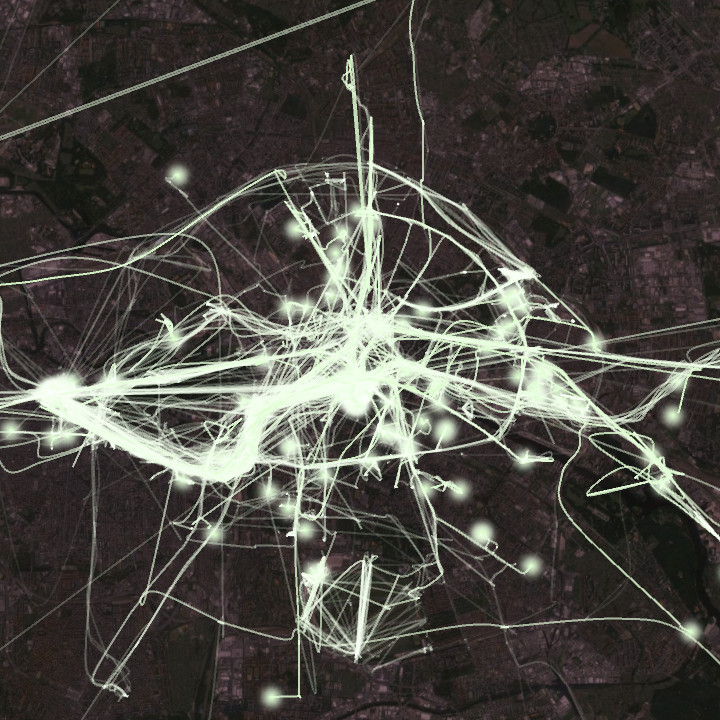
According to Google’s Data Liberation Front (and German privacy laws), users are able to download a complete record of their data from the Google servers. This service is implemented as Google Takeout. I downloaded my Location History data of the last few months and created an animation using Processing. My movement patterns of all recorded days are superposed in one video.
If you want to create one of these by yourself you could download the source code at GitHub.
Data Acquisition
If location history is enabled on your Android device, you can easily download a large JSON file including every single ever recorded location sample of you. This file can easily get tens of megabytes large. Besides the location data, a map image of the area is also needed. I used the Copy Image function of Google Earth to export this nice view of view of Berlin:

The image also displays an Image Overlay of a calibration grid, that was added to the export. Google Earth allows to add overlays at given geological coordinates. A little 4-point-calibration gives some good results.
Calibration
Google Earth and the Location History protocol use two different notations to express geological coordinates. While in Google Earth they look like this: 52°33’20.39″N, 13°19’17.47″E (degrees°minutes’seconds”), they would appear looking like this: 52.555663889, 13.321519444 (decimal) in the Location History. You can easily convert between them using: decimal = degrees + minutes/60 + seconds/3600.
To match the geological coordinates \(p\) from the Takeout JSON with pixel coordinates \(p’\) of our map image, we have to apply a calibration. Assuming a projective mapping \(H\) between both coordinate systems exist, which should approximately be the case for relatively small areas of the globe, we can formulate the following equation:
\[ \begin{aligned}
p’ & = H \cdot p \\
\begin{pmatrix} x’ \\ y’ \\ w’ \end{pmatrix} & = \begin{pmatrix} h_{11} & h_{12} & h_{13} \\ h_{21} & h_{22} & h_{23} \\ h_{31} & h_{32} & 1 \end{pmatrix} \cdot \begin{pmatrix} x \\ y \\ 1 \end{pmatrix} \\
\end{aligned}
\]
To convert the homogeneous pixel coordinates \(p’\) to Euclidean coordinates \( \left( X, Y \right) \), we use the following equations:
\[ \begin{aligned}
X & = \frac{x’}{w’} \\
Y & = \frac{y’}{w’} \\
\end{aligned}
\]
Expressing these using \(H\) and the geological coordinates \(\left(x,y\right)\) gives the following equations:
\[ \begin{aligned}
X & = h_{11} x + h_{12} y + h_{13} – X h_{31} x – Y h_{32} y \\
Y & = h_{21} x + h_{22} y + h_{23} – X h_{31} x – Y h_{32} y \\
\end{aligned}
\]
In order to determine \(H\) we reformulate them to:
\[ \begin{aligned}
\begin{pmatrix} X \\ Y \\ \vdots \\ \vdots \\ \vdots \end{pmatrix} & =
\begin{pmatrix} x & y & 1 & 0 & 0 & 0 & -Xx & -Yy \\ 0 & 0 & 0 & x & y & 1 & -Xx & -Yy \\ & & & & \vdots & & & \\ & & & & \vdots & & & \\ & & & & \vdots & & & \end{pmatrix} \cdot
\begin{pmatrix} h_{11} \\ h_{12} \\ h_{13} \\ h_{21} \\ h_{22} \\ h_{23} \\ h_{31} \\ h_{32} \end{pmatrix} \\
b & = A \cdot h
\end{aligned}
\]
Using four known corresponding points \(\left(x,y\right)\) and \(\left(X,Y\right)\), each adding two equations to the system, we can solve for all eight unknown parameters of \(H\):
\[ \begin{aligned}
A^{-1} \cdot b & = h
\end{aligned}
\]
The following OCTAVE code does the job. The matrices x and X hold our four corresponding point pairs of geological and pixel coordinates determined from the above overlay image.
% input quad
x = [
		52.555663889 13.321519444
		52.555663889 13.426994444
		52.491488889 13.426994444
		52.491488889 13.321519444
	]

% output quad
X = [
		516 223
		1046 192
		1083 727
		532 759
	]

% design matrix
A = [];
for i = 1:size(x,1)
	A = [A;
		x(i,1) x(i,2) 1, 0 0 0, -X(i,1)*x(i,1) -X(i,1)*x(i,2)
		0 0 0, x(i,1) x(i,2) 1, -X(i,2)*x(i,1) -X(i,2)*x(i,2)
	];
end

% homography
h = inv(A) * X'(:);
H = reshape([h;1],3,3)'

csvwrite('homography.csv', H);
You could also do the same directly in Java / Processing using LUD, a minimalistic class for LU decomposition on 2d arrays:
// input quad
double[][] x = {
		{ 52.555663889, 13.321519444 },
		{ 52.555663889, 13.426994444 },
		{ 52.491488889, 13.426994444 },
		{ 52.491488889, 13.321519444 },
};

// output quad
double[][] X = {
		{ 516, 223 },
		{ 1046, 192 },
		{ 1083, 727 },
		{ 532, 759 },
};

// equation system to solve for h
double[][] A = new double[8][];
double[][] b = new double[8][];
for (int i=0; i<4; i++) {
	// coefficients
	A[2*i+0] = new double[] { x[i][0], x[i][1], 1, 0, 0, 0, -X[i][0]*x[i][0], -X[i][0]*x[i][1] };
	A[2*i+1] = new double[] { 0, 0, 0, x[i][0], x[i][1], 1, -X[i][1]*x[i][0], -X[i][1]*x[i][1] };
	// constant terms
	b[2*i+0] = new double[] { X[i][0] };
	b[2*i+1] = new double[] { X[i][1] };
};

// solve Ah = b
double[][] h = new LUD(LUD.copy(A)).solve(b);

// reshape
double[][] H = {
		{ h[0][0], h[1][0], h[2][0] },
		{ h[3][0], h[4][0], h[5][0] },
		{ h[6][0], h[7][0], 1 }
};
